
Stacking Triangles for Fun and Profit
One thing you may have noticed about the trigonometric functions sine and cosine is that they seem to have no agreed upon definition. Or rather, different authors choose different definitions as the starting point, mainly based on convenience. This isn’t problematic or even particularly unusual in mathematics - as long as we can derive any of the other forms from any starting point, it makes little theoretical difference which we start from since they’re all equivalent anyway.
The most common starting points are the series definitions, the solution to an initial value problem involving ordinary differential equations, or using complex numbers as Euler’s formula. You can find detailed descriptions of these on the Wikipedia page. These are all fine starting points as far as they go, and as I said before they are all equivalent.
What struck me as odd when I was an undergraduate, and still strikes me to this day, is that none of these are the obvious trigonometric definitions about the opposite and adjacent sides of a right triangle. Aren’t axioms and definitions supposed to be obvious, so obvious and self-evident they can’t be doubted? So why are we using a highly non-obvious formulation as our definition, and then backing into the intuitive form as a theorem? The answer is actually simple - the proofs are slightly shorter when we do it that way.
However, I never liked this approach because it’s very much like pulling a rabbit out of a hat, or perhaps more like pulling a “previously prepared” turkey out of the oven on a cooking show. It gives students a completely backward impression of how mathematics is done. We don’t start from intuitive definitions and work on them until we can understand them more deeply or connect them to other structures; no, we simply write down a bizarre and unmotivated equation and show it has the desired properties, with no mention of how anyone thought it up in the first place. This often leads to shorter, more elegant proofs but at the cost of completely failing to teach the student how to actually “do” mathematics.
I mean, look at this thing:
\[ \sin(x) = \sum_{n=0}^{\infty} \frac{(-1)^n}{(2n+1)!} x^{2n+1} \]
Anyone who looks at that and says, “yes, that’s a self-evident definition” is either lying or Ramanujan.
The differential equation definition is almost as bad. The equations themselves are fairly simple:
\[
\begin{align}
\frac{d^2y}{dt^2} &= -y \\\
y(0) &= 0 ,&
y’(0) &= 1
\end{align}
\]
The problem is that we have to rely on the ODE existence and uniqueness theorem which is non-trivial to prove; the most common proof involves invoking the Banach fixed point theorem. That seems like a weirdly technical approach to defining what should be an elementary concept.
What would be nice would be to start from the intuitive, geometric definition:
\[
\begin{align}
\sin(\theta) &= \frac{\text{opposite}}{\text{hypotenuse}} \\\
\cos(\theta) &= \frac{\text{adjacent}}{\text{hypotenuse}}
\end{align}
\]
and derive the analytic definitions by working forward. I think I’ve found a clear and unambiguous way to explain this at the undergraduate level. Briefly, we’ll prove the angle addition formulas using geometric methods, then show how this leads immediately to the other results.
Since we’re interested in establishing a foundation for sine and cosine from geometric principles, we have to establish some ground rules. It’s of crucial importance that you ignore everything you already know about these functions. Yes, I know you can prove this stuff more easily from Euler’s formula. Yes, I know there a dozen different ways to prove any of these. For the moment, pretend like you don’t know anything about sine and cosine except the geometric definitions, and we won’t use anything unless we’ve proved it earlier. The structure of the proofs will be as follows:
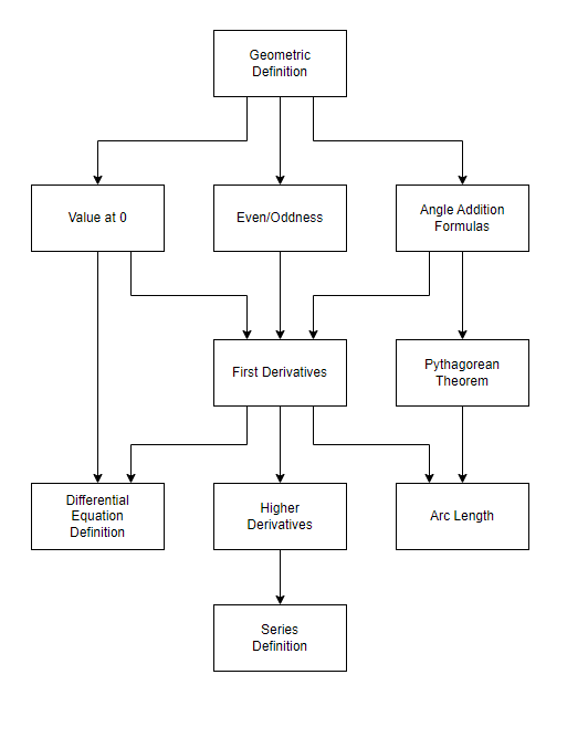
As the goal is to ground everything on the geometric definition in an easy-to-follow way, jumping ahead and using theorems before we’ve established that foundation defeats the purpose.
Notation
In the first draft of this proof, I left points unlabeled and simply referred to “the middle triangle” or the “right angle in the top triangle” and so on. The idea was to keep things simple for a broad audience but I quickly found it was very hard to follow. Instead, we’ll use the conventional notation, which I’ll briefly review here.
We use upper case roman letters such as $A$ or $B$ to label points. The line segment connecting two points is written $\overline{AB}$. The triangle with vertices $A$, $B$, and $C$ is written $\triangle ABC$. Even though the notation symbol shows an equilateral triangle, the triangle in question doesn’t have to be. I’ll write “The right triangle $\triangle ABC$” if it’s important to specify that the triangle is a right triangle.
The above are all fairly self-explanatory, but the last bit of notation can be confusing if you don’t know exactly what it means. To describe the angle at $B$ between $\overline{AB}$ and $\overline{BC}$, we write $\angle ABC$.
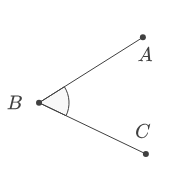
$\angle ABC$ is always equal to $\angle CBA$, but $\angle BAC$ or $\angle ACB$ refer different angles located at a different part of the diagram. To locate an angle $\angle ABC$ in the diagram, first look for the point labeled with the middle letter $B$. Then imagine lines connecting $B$ to $A$ and $C$ - the angle referred to is the angle between those lines.
I know this notation takes some getting used to, but it allows us to unambiguously refer to angles on a cluttered diagram.
Geometric Proof of Angle Addition Formulas
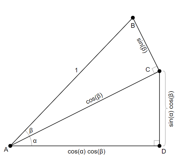
We set up the problem by simply stacking two right triangles on top of each other.
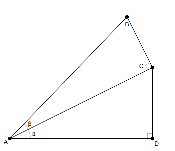
Let’s define $\overline{AB}$ to have a length of 1. $\overline{AB}$ is hypotenuse of the right triangle $\triangle ABC$. Since the hypotenuse is length 1, the lengths of opposite and adjacent sides are simple $\sin(\beta)$ and $\cos(\beta)$ respectively.
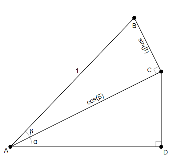
We can do the same thing for the triangle $\triangle ACD$ and angle $\alpha$ but with the twist that hypotenuse of this triangle is no longer 1 but instead $\cos(\beta)$. Therefore, the lengths of the opposite and adjacent sides have to each be multiplied by $\cos(\beta)$.
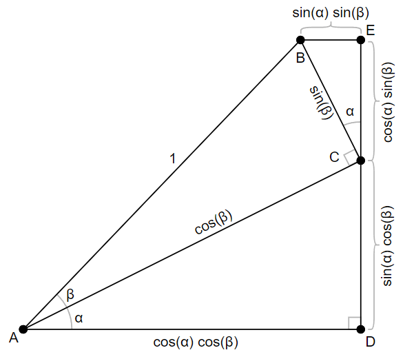
Let’s add another triangle to our diagram by extending $\overline{CD}$ out in a straight line and drawing a perpendicular line through the point $B$. This gives us the triangle BCE. Since $\overline{BE}$ is perpendicular to $\overline{EC}$ it is in fact a right triangle.
Now, the line $\overline{EC}$ is perpendicular to $\overline{AD}$, and the line $\overline{BC}$ is perpendicular is $\overline{AC}$, so the angle $\angle BCE$ is the same as the angle $\angle CAD$ which we called $\alpha$.
Now that we know the hypotenuse and one angle of the right triangle $\triangle BCE$ we can once again use the definitions of sine and cosine to label the lengths of the opposite and adjacent sides.
We’ll do something similar for the last triangle. We’ll draw a line perpendicular to $\overline{AD}$ through $A$ and extend it up to point $F$ where it intersects the extension of $\overline{BE}$. $\overline{FE}$ and $\overline{AD}$ are parallel (because they are both perpendicular to $\overline{AF}$) therefore $\angle FBA$ is equal to $\angle BAD$ which is the sum of $\alpha$ and $\beta$. So we can label this angle $\alpha+\beta$. For the fourth and final time, we’ll use the definition of sine and cosine to label opposite and adjacent sides of the right triangle $\triangle FAB$. Note that this is where the expressions $\cos(\alpha + \beta)$ and $\sin(\alpha + \beta)$ enter the proof.
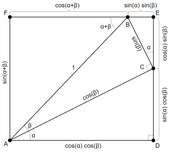
So far, everything has been construction - adding triangles and chasing angles to label edge lengths. But now the diagram is complete, and we can easily read off the angle addition formulas by equating opposite sides. Note that $FEAD$ forms a rectangle; $\overline{FE}$ and $\overline{AD}$ are parallel which proves $\overline{AF}$ and $\overline{DE}$ are equal; likewise $\overline{AF}$ and $\overline{ED}$ are parallel, which proves $\overline{FE}$ and $\overline{AD}$ are equal. All we have to do now is equate opposite pairs of sides:
\[
\begin{align}
\cos(\alpha+\beta) + \sin(\alpha) \sin(\beta) = \cos(\alpha) \cos(\beta) \\\
\sin(\alpha+\beta) = \sin(\alpha) \cos(\beta) + \cos(\alpha) \sin(\beta)
\end{align}
\]
Finally, we rearrange these slightly to put them in the canonical form of the angle addition formulas:
\[
\begin{align}
\cos(\alpha+\beta) &= \cos(\alpha) \cos(\beta) - \sin(\alpha) \sin(\beta) \\\
\sin(\alpha+\beta) &= \sin(\alpha) \cos(\beta) + \cos(\alpha) \sin(\beta)
\end{align}
\]
Pythagorean Theorem
OK, now that we have the angle addition formulas, let’s put them to work.
First, we’d like sine and cosine to trace out a unit circle; in other words, we want to make sure that $\sin^2(\theta) + \cos^2(\theta) = 1$ for all angles $\theta$.
There are lots of ways to prove this, but the angle addition formula provides one of the neatest approaches. Instead of adding two separate angles $\alpha$ and $\beta$, we’ll use $\theta$ and $-\theta$. These two angles sum to zero, so we have:
\[
\begin{align}
1 &= \cos(0) \\\
&= \cos(\theta - \theta) \\\
&= \cos(\theta)\cos(-\theta) - \sin(\theta)\sin(-\theta) \\\
&= \cos(\theta)\cos(\theta) + \sin(\theta)\sin(\theta) \\\
&= \cos^2(\theta) + \sin^2(\theta)
\end{align}
\]
Here, we additionally used the fact that sine and cosine are odd and even functions respectively, so $\cos(-x) = \cos(x)$ and $\sin(-x) = - \sin(x)$.
That means that the Pythagorean theorem is actually an immediate corollary of the angle addition formula for cosine.
Derivatives
Another neat thing we can do with the angle addition formulas is calculate the derivatives of sine and cosine. This is because the limit definition of derivative includes a term with $f(x+h)$ which we can handle with the formulas.
\[
\begin{align}
\frac{d}{dx} \sin(x) &= \lim_{h \to 0} \frac{\sin(x + h) - \sin(x)}{h} \\\
\end{align}
\]
\[ \begin{align} &= \lim_{h \to 0} \frac{\sin(x)\cos(h) + \cos(x)\sin(h) - \sin(x)}{h} \end{align} \]
By considering a triangle with hypotenuse 1 and a very small “opposite” side, it’s not hard to see geometrically that $\sin(h) \approx h$ and $\cos(h) \approx 1$ when $h$ is close to zero. Therefore we have:
\[ \begin{align} \frac{d}{dx} \sin(x) &= \lim_{h \to 0} \frac{\sin(x) + \cos(x) h - \sin(x)}{h} \end{align} \]
\[ \begin{align} &= \lim_{h \to 0} \frac{\cos(x) h}{h} \end{align} \]
\[ \begin{align} &= \cos(x) \end{align} \]
The equivalent argument for $\cos(x)$ is:
\[ \begin{align} \frac{d}{dx} \cos(x) &= \lim_{h \to 0} \frac{\cos(x + h) - \cos(x)}{h} \end{align} \]
\[ \begin{align} &= \lim_{h \to 0} \frac{\cos(x)\cos(h) - \sin(x)\sin(h) - \cos(x)}{h} \end{align} \]
\[ \begin{align} &= \lim_{h \to 0} \frac{\cos(x) - \sin(x) h - \cos(x)}{h} \end{align} \]
\[ \begin{align} &= \lim_{h \to 0} \frac{-\sin(x) h}{h} \end{align} \]
\[ \begin{align} &= -\sin(x) \end{align} \]
Once we know these first derivatives, computing higher derivates is straightforward. For example, the second derivatives are:
\[ \frac{d^2}{dx^2} \sin(x) = \frac{d}{dx} \cos(x) = -\sin(x) \]
\[ \frac{d^2}{dx^2} \cos(x) = \frac{d}{dx} -\sin(x) = -\cos(x) \]
With just these second derivatives, we can already motivate the initial value problem ODE definition of sine and cosine.
It’s equally obvious that we can continue the process indefinitely, alternating between sine and cosine. Since we know $\sin(0) = 0$ and $\cos(0) = 1$, we can evaluate all derivatives of sine and cosine at zero, allowing us to calculate the Maclaurin series. This gives us the series form.
Arc Length
The above shows that sine and cosine trace out a unit circle, but there is one final thing we need to show to fully connect the geometric and analytic definitions.
The formula for arc length is:
\[ L = \int_{a}^{b} \sqrt{\left(\frac{dx}{dt}\right)^2 + \left(\frac{dy}{dt}\right)^2} \, dt \]
Let’s write down the equations for the unit circle in parametric form. Luckily,
we already worked out the first derivatives:
\[
\begin{align}
x(t) = \cos(t), & \frac{dx}{dt} = -\sin(t)
\end{align}
\]
\[ \begin{align} y(t) = \sin(t), & \frac{dy}{dt} = \cos(t) \end{align} \]
Then, substituting these into the arc length formula: \[ L = \int_{0}^{\theta} \sqrt{(-\sin(t))^2 + (\cos(t))^2} \, dt \]
Simplifying inside the square root: \[ L = \int_{0}^{\theta} \sqrt{\sin^2(t) + \cos^2(t)} \, dt \]
Since we showed above that $\sin^2(t) + \cos^2(t) = 1$ for all $t$, this further simplifies to: \[ L = \int_{0}^{\theta} 1 \, dt \]
Integrating from $0$ to $\theta$: \[ L = \left. t \right|_{0}^{\theta} = \theta - 0 = \theta \]
This tells us that the parameter $t$ we used is equal to the arc length along the unit circle; in other words, the angle expressed in radians.
Conclusion
We’ve shown that all of usual definitions of sine and cosine can be derived from the geometric definition, and that this can be made elementary if we start by proving the angle addition formulas using geometric arguments. The geometric proof itself is quite beautiful and easy to remember as it is simply a matter of stacking two triangles, building a rectangle around them, and equating the opposing sides. We offer this as a more pedagogically sound and historical accurate way to motivate the various definitions of sine and cosine.